Blog — Mathematical principles

Elements of neural networks

This text is inspired by Andrej Karpathy’s micrograd. Below, we will build a neural network from scratch, explaining each of its elements in detail.

The Derivative Demonstrated Geometrically

Neural networks are gigantic mathematical functions. The distinctive feature of these functions, which catalyze much of what is now called “artificial intelligence” (although, more strictly, we should speak of “deep learning”), is that they can “learn” to refine, optimize, and generalize the “rules” (parameters) that compose them. Such a learning process consists of the iteration of mathematical operations from differential and vector calculus. Therefore, to formulate a neural network, we will first try to intuitively understand the derivative: the mathematical core of learning.

For this purpose, we will construct the derivative from scratch, using only a few basic notions of geometry.

In geometry, we call “slope” the value of the inclination of a line. Conceptually, the slope can be interpreted as the proportion of change between the variables x and y of the line. In other words, the slope measures how much x influences the value of y, or how much y changes as we advance in x. Let’s suppose, for example, the line of a function that we can define as f(x, b) = x \cdot b, where:

x = np.arange(0, 21, 2)
b = 5
def f(x, b): return x*b
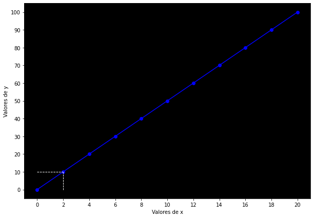
y = f(x, b)

In simpler terms, the function is a multiplication between x (numbers from 0 to 20 in intervals of 2) and b (i.e., 5).

Now, how can I know how much each value of x is influencing each value of y? That is, if I go from x=2 to x=4, what happens to y? y moves from 10 to 20, that is, five times x: 5 \times 2 = 10. And if I go from x=4 to x=6, that is, if I advance two “steps” in x, y again advances five times what I advanced in x, going from 20 to 30.

In that sense, the proportion between x and y is 5. 5 is the number that determines each value of y from x or, in other words, 5 is the “force” with which x influences y. This intuition is key, but at the same time it is obvious because the definition of my function (that is, each value of y) indicates that I must multiply x by 5. By calculating the slope, it is as if we did not know this number and had to deduce it mathematically.

The slope formula offers us a general method to calculate this proportion or force we are talking about¹:

Slope = \frac{y_2 - y_1}{x_2 - x_1} = \frac{\Delta y}{\Delta x}

So the formula just tells us that we must take any two points of x and y to calculate the slope. For example, if we consider the values of the point denoted by the dashed lines in the previous graph, such that x_1 = 2, y_1 = 10, we can take the next point to calculate the slope or inclination of the line, so that:

Slope = \frac{20 - 10}{4 - 2} = \frac{10}{2} = 5

But linear functions (that is, straight lines) by definition have the same inclination at all their points or segments. Let’s check this by changing our x_2, y_2:

Slope = \frac{y_2 - y_1}{x_2 - x_1} = \frac{60 - 10}{12 - 2} = \frac{50}{10} = 5

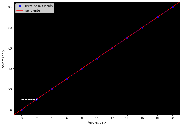
Naturally, the slope remains the same. Now let’s reiterate, what exactly does the number five mean? That for every step we take in x, y advances five times more. In other words, y is the result of multiplying x by five; or x influences y with a “force” of five times itself; or x transforms y with a force of five times itself.

The slope is identical to the line because, as we were saying, the line has the same inclination (slope) at all its points. Now, the problem with the slope is that this property is at the same time a fundamental limitation: the slope is only valid for a straight line or linear function.

Since non-linear functions do not have the same inclination at all their points, we cannot speak of the “inclination” or the “slope of a non-linear function”. Let’s visualize this with a quadratic function, where my x values now go from 0 to 5.99. Let’s also say that I’m interested in knowing the inclination or “slope” of the function when x=5:

x = np.arange(0, 6, 0.0001)
def nonlinear(x): return x**2
y = nonlinear(x)

slope = (5**2 - 2**2) / (5 - 2)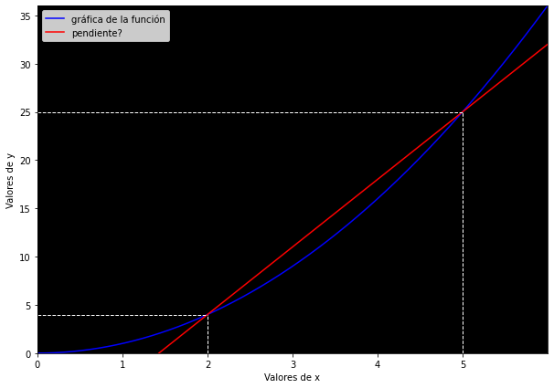

To calculate the inclination of the function (i.e., the blue curve) when x=5, I have used the slope formula taking as reference the points x_1=2, x_2=5, such that:

Slope = \frac{y_2 - y_1}{x_2 - x_1} = \frac{25 - 4}{5 - 2} = \frac{21}{3} = 7

But the reality is that my function did not change in that proportion with respect to the point x=5: that slope of 7 corresponds to the secant² that crosses the function, not to the “slope” of the point x=5. The graph shows that the result is inaccurate: it is clear that the function has a different inclination than that of the red line³.

Besides the fact that the function has multiple “slopes” (because its inclination always changes), these “slopes” are inexact, since they do not precisely measure the impact (or inclination) of a single point in the function, but rather the slope formula necessarily gives us the inclination of a line drawn between two values of x and two values of y. Since the function we are dealing with now is curved, the points of x and y we take are not satisfactory because they denote a line, not a curve. In that sense, the result is biased.

So, how can I find the true impact of x on y? We can think of the following trick: if the slope of the secant, although erroneous, approaches in some way our desired value, couldn’t we make a smaller secant, such that it would be more similar to the point we are interested in? That is, if we took the slope of the distance between two points of x closer to each other, that should give us a better approximation to the correct result, right?

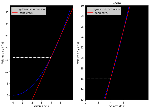
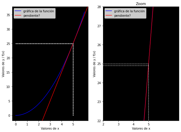
Graphically we can verify that we have obtained a much better result: the secant we drew has an inclination similar to that of the curve of the function. But the dashed lines (which denote the points we have taken as reference to calculate the slope) indicate that we can still improve, taking as reference coordinates closer to each other.

Well, before continuing to experiment, let us already advance that this line of reasoning is precisely what gave rise to the derivative⁴. The trick is this: we can calculate the slope of secant lines that are increasingly smaller and more similar to our point, obtaining increasingly better results. Moreover, we can arrive at calculating the slope of an infinitely small line, so small that it would be almost identical to the point, and the slope of that infinitely small line would be equal to the slope of the point. In that same sense, we could even say (and in fact this is done in the mathematical field) that we are calculating the slope of a tangent line to the point, since its slope would be equal to that of an infinitely small secant that merges with the point.

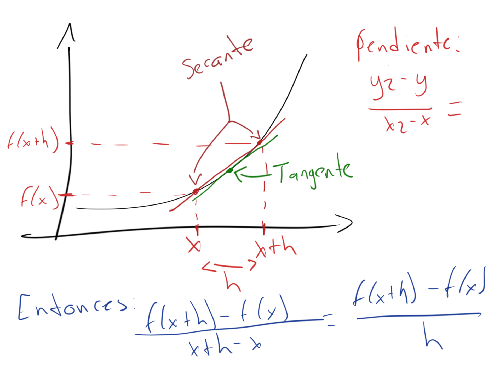
Using the slope formula to put our intuition into practice:

Slope = \frac{y_2 - y_1}{x_2 - x_1} = \frac{f(x+h) - f(x)}{(x+h) - x} = \frac{f(x+h) - f(x)}{h}

As I was saying, ideally we want the distance h to be as small as possible, that is, as close to 0 as possible (without being 0, since we need a distance between two x’s to have a line and thus be able to obtain its slope, since a point has no slope). To express this idea, we will use the expression \lim _{h \rightarrow 0}, that is, “when h is so small that it approaches 0” or, more strictly, “the limit of the function when h tends to 0”. Such that:

\lim _{h \rightarrow 0} \frac{f(x+h) - f(x)}{h}

But now we are no longer talking about a slope exactly, but rather we are altering it to achieve a different result⁵. We will call this new concept the “derivative”:

Derivative = \lim _{h \rightarrow 0} \frac{f(x+h) - f(x)}{h}

In practice it is also usually written as \frac{dy}{dx}, or f'(x)⁶.

Applied to our problem, we can use it like this:

\frac{dy}{dx} =\lim _{h \rightarrow 0} \frac{f(x+h) - f(x)}{h} = \frac{(5+0.001)^2 - 5^2}{0.001} = 10.00

Programmatically:

def derivative(f, x):
  h = 0.001
  return (f(x+h) - f(x)) / h

derivative(nonlinear, 5)

~ 10.001000000002591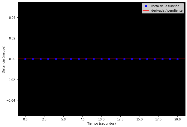

We have finally discovered that when x=5, x “influences” y with a “force” of 10⁷. Analytically, we can verify it this way:

\begin{gather*} \frac{dy}{dx} =\lim _{h \rightarrow 0} \frac{(x+h)^2 - x^2}{h} = \lim _{h \rightarrow 0} \frac{(x+h)(x+h) - x^2}{h} = \lim _{h \rightarrow 0} \frac{x^2 + xh + hx + h^2 - x^2}{h} \\ = \lim _{h \rightarrow 0} \frac{2xh + h^2}{h} = \lim _{h \rightarrow 0} \frac{h(2x + h)}{h} = \lim _{h \rightarrow 0} (2x + h) = 2x + 0 = 2x \end{gather*}

Now, we can generalize this expression under the formula nx^{n-1}, that is, when f(x) = x^2 and x=5, then:

\begin{gather*} 2x = 2(5) = 10 \\ nx^{n-1} = 2(5)^{2-1} = 10 \end{gather*}

In sum, 10 is effectively the proportion or force with which x influences y, 10 is the derivative of y with respect to x when x=5. And, as we have seen, we can obtain this result in different ways: applying the formula, programmatically, geometrically, and analytically or algebraically. In general, every formula or mathematical expression has a rational background like the ones we have carried out, although more often than not some further logical-mathematical developments are required to generalize them.

Returning to our topic, we can conclude that, conceptually, the derivative (like the slope) measures the proportion or magnitude of the change that a variable causes in the result of a function. Let’s say that the derivative measures the force with which a variable influences, at a given point, the result of a function⁸.

But what is the derivative for?

Let us imagine that we have two variables: x = -2 and y = 3. The function f(x, y) multiplies them and its result is -6. However, we want to alter that result so that it is 0 and we have a constraint: the only way to do so is through the input variables⁹.

If we remember the lesson learned about derivatives, we might think of using them to solve this problem: since the derivative tells me the impact that an input variable has on the function, would it be possible to use it to alter the result of the function? That is, if the derivative tells me the magnitude of the impact that a variable has on the result, then I should be able to use that information to influence the result more efficiently.

Tinygrad

To better understand the proposed solution, we will programmatically create the Value class, that is, we will formulate a structure that allows us to define, modify, and operate with numbers. For now, each Value will have the following properties: a data, a pair of previous values in case the data was generated through an operation (for example, 2 and 2 in case they were multiplied to generate the number 4), the operation that generated said value (in our example, multiplication) and a label in case we want to associate our data with a variable. For now, we will only have addition, multiplication, subtraction, and division operations:

class Value:
  def __init__(self, data, _children=(), _op='', label=''):
    self.data = data
    self._prev = set(_children)
    self._op = _op
    self.label = label

  def __add__(self, other):
    other = other if isinstance(other, Value) else Value(other)
    out = Value(self.data + other.data, (self, other), '+')
    return out

  def __mul__(self, other):
    other = other if isinstance(other, Value) else Value(other)
    out = Value(self.data * other.data, (self, other), '*')
    return out

  def __sub__(self, other):
    return self + (-other)

  def __truediv__(self, other):
    return self * other**-1

  def __neg__(self):
    return self * -1

  def __repr__(self):
    return f'Value={self.data}'

We will use a more challenging problem than a simple multiplication:

a = Value(-2.0, label='a')
b = Value(3.0, label='b')
c = a*b; c.label = 'c'
d = Value(10.0, label='d')
e = c + d; e.label = 'e'
f = Value(-3.0); f.label = 'f'
L = f * e; L.label = 'L'

We can visualize this computational graph:

As we were saying, we intuitively believe that the derivative can help us: with the derivative we know what impact each variable has on the final result L. In that sense, what we will have to do first is calculate the derivative of L with respect to each variable¹⁰.

In principle, the derivative of L with respect to itself is 1: although it may sound absurd and obvious at the same time, the change in L is proportional (identical) to itself. Now, the derivative of L with respect to f and e we can find out with the formula we have been using:

def derivative():
  h = 0.000001
  # Original function
  a = Value(-2.0, label='a')
  b = Value(3.0, label='b')
  c = a*b; c.label = 'c'
  d = Value(10.0, label='d')
  e = c + d; e.label = 'e'
  f = Value(-3.0); f.label = 'f'
  L1 = f * e

  # Function with increment h
  a = Value(-2.0, label='a')
  b = Value(3.0, label='b')
  c = a*b; c.label = 'c'
  d = Value(10.0, label='d')
  e = c + d; e.label = 'e'
  e.data += h
  f = Value(-3.0); f.label = 'f'
  L2 = f * e

  print((L2 - L1) / h)

derivative()

~ Value=-3.0

The derivative of the function L with respect to e is approximately -3. By this point, we will have noticed a pattern: when we differentiate a multiplication, the partial derivative with respect to the multiplicand is the multiplier. In this case, L is the result of multiplying e with f. We saw that the derivative with respect to e is -3, that is f. We can induce, empirically and by symmetry, that the derivative with respect to f is e, that is 4.

Let us also demonstrate analytically what we have been saying. Using our mathematical formula, we have:

\frac{\partial L(e, f)}{\partial e}=\lim _{h \rightarrow 0}{\frac{L(e + h, f)-L(e, f)}{h}} = {\frac{(e + h) \cdot f - e \cdot f}{h}} = {\frac{ef + hf - ef}{h}} = {\frac{hf}{h}} = f

And although the notation may appear complex, in reality we are only adding, multiplying, subtracting, and dividing.

Now that we have this information, we want to continue to the previous node: the derivatives with respect to c and d. But here there is a subtlety that, well understood, will give us the key to neural networks: we must obtain the derivative of L with respect to c and d, not the derivative of e with respect to them. So, how can we find out the impact that c and d have on L through e? To make this calculation, only a fairly simple intuition is needed¹¹.

The Chain Rule: Backpropagation

Let’s borrow George Simmons’s analogy: if a bicycle is twice as fast as a person running, and a car is four times faster than a bicycle, then the car is 2 \times 4 = 8 times faster than a person running.

Similarly, if we want to know the influence that c has on L, we only need to obtain the derivative of e with respect to c, and multiply it by the derivative of L with respect to e. That is, we must multiply the force of c on e and that of e on L to know with how much force c influences L. The same applies to d and all the others; this rule is called the “chain rule” (and through it “backpropagation” is performed in the field of artificial intelligence).

Now, to obtain the derivative of e with respect to c, let’s remember another pattern we saw: in an addition, the derivative gave us 1 as a result because the function advanced in the same proportion as the variable advanced. Let’s verify:

def deriv_e(c, d):
  return (((c+0.00001)+d) - (c+d)) / 0.00001

deriv_e(-6, 10)

~ 1.0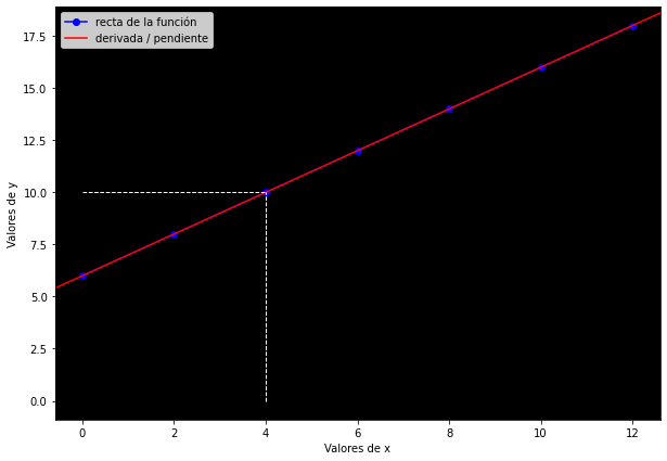

Indeed, the result is approximately 1. By symmetry again, we understand that the derivative of e with respect to d is also 1. Analytically:

\frac{\partial e(c, d)}{\partial d}=\lim _{h \rightarrow 0}{\frac{e(c, d+h)-e(c, d)}{h}} = {\frac{(c + d + h) - (c + d)}{h}} = {\frac{(c+d) + h - (c+d)}{h}} = {\frac{h}{h}} = 1

And now that we have both partial derivatives, we can multiply them following the chain rule: 1 \times -3 = -3. Thus, the derivative of L with respect to c and d is -3. In mathematical terms, we have done something equivalent to:

\frac{dz}{dx} = \frac{dz}{dy} \cdot \frac{dy}{dx}

Where z depends on y and, in turn, y depends on x.

Finally, we must do the same to obtain the derivatives with respect to a and b. Then, given the pattern we had discovered, the derivative of c with respect to a is b, that is 3, and vice versa: the derivative with respect to b is a, that is -2. But let’s remember: these “local” derivatives are of the function c, and we are interested in the derivative of L, that is, the magnitude of the influence that a and b have on L. To know this, we must again apply the chain rule and multiply the derivatives we have by the derivative of L with respect to c. Then, the partial derivative of L with respect to a is 3 \times -3 = -9, while the partial derivative with respect to b is -2 \times -3 = 6¹².

Now that we have these values, we can optimize our code to account for them. In practice, nobody calculates derivatives manually as we did, since it would be an eternal task; but we have already learned the patterns to calculate them, so we can implement them in our code so that they are calculated automatically:

import math

class Value:
  def __init__(self, data, _children=(), _op='', label=''):
    self.data = data
    self.grad = 0.0
    self._backward = lambda: None
    self._prev = set(_children)
    self._op = _op
    self.label = label

  def __add__(self, other):
    other = other if isinstance(other, Value) else Value(other)
    out = Value(self.data + other.data, (self, other), '+')

    def _backward():
      self.grad += 1.0 * out.grad
      other.grad += 1.0 * out.grad
    out._backward = _backward

    return out

  def __mul__(self, other):
    other = other if isinstance(other, Value) else Value(other)
    out = Value(self.data * other.data, (self, other), '*')

    def _backward():
      self.grad += other.data * out.grad
      other.grad += self.data * out.grad
    out._backward = _backward

    return out

  def __pow__(self, other):
    assert isinstance(other, (int, float))
    out = Value(self.data**other, (self,), f'**{other}')

    def _backward():
      self.grad += other * (self.data ** (other - 1)) * out.grad
    out._backward = _backward

    return out

  def tanh(self):
    t = (math.exp(2*self.data) - 1) / (math.exp(2*self.data) + 1)
    out = Value(t, (self,), 'tanh')

    def _backward():
      self.grad += (1 - t**2) * out.grad
    out._backward = _backward

    return out

  def backward(self):
    topo = []
    visited = set()
    def build_topo(v):
      if v not in visited:
        visited.add(v)
        for child in v._prev:
          build_topo(child)
        topo.append(v)
    build_topo(self)

    self.grad = 1
    for node in reversed(topo):
      node._backward()

  def __neg__(self):
    return self * -1

  def __sub__(self, other):
    return self + (-other)

  def __truediv__(self, other):
    return self * other**-1

  def __repr__(self):
    return f'Value={self.data}'

Since our loss function is positive, we want to decrease it. If the gradients indicate the direction in which we can increase the result of a function, then in this case we want to go in the opposite direction of the gradient, as that would result in a decrease of the function’s result. To do this, we will add value to the variables in the inverse direction of the gradient.

Multilayer Perceptron

Previously, we built a kind of neuron; however, the power of a neural network is that it has millions of neurons, all optimizing their values to give us the result we want (in our example: 0)¹³.

Next, we will build a neural network called a “multilayer perceptron” (MLP) that will allow us to solve practical problems. As an example, we will train it to identify sarcasm in movie reviews.

To detect sarcasm in the reviews that users give about a movie, we could take as a basis two variables: the sentiment (with values from 1 to 5, where 5 is a positive sentiment and 1 a negative one) and the assigned rating (also with values from 1 to 5). The result should be 1 for sarcasm and 0 for absence of sarcasm. For example:

• Great, I love watching a horror movie with the typical plot. Rating: 2/5.

In this case, the sentiment is positive (it uses expressions like “great”, “I love”), but the review is negative, so we can establish an inverse proportionality relationship between both variables to detect sarcasm: if the rating is low but the sentiment is “high”, then there is sarcasm (i.e., sarcasm =1).

import random

class Neuron:
  def __init__(self, nin):
    self.w = [Value(random.uniform(-1,1)) for i in range(nin)]
    self.b = Value(random.uniform(-1,1))

  def __call__(self, x):
    act = sum((wi*xi for wi, xi in zip(self.w, x)), self.b)
    out = act.tanh()
    return out

  def parameters(self):
    return self.w + [self.b]

class Layer:
  def __init__(self, nin, nout):
    self.neurons = [Neuron(nin) for _ in range(nout)]

  def __call__(self, x):
    outs = [n(x) for n in self.neurons]
    return outs[0] if len(outs) == 1 else outs

  def parameters(self):
    return [p for n in self.neurons for p in n.parameters()]

class MLP:
  def __init__(self, nin, nouts):
    sz = [nin] + nouts
    self.layers = [Layer(sz[i], sz[i+1]) for i in range(len(nouts))]

  def __call__(self, x):
    for layer in self.layers:
      x = layer(x)
    return x

  def parameters(self):
    return [p for layer in self.layers for p in layer.parameters()]

We will give our model four training inputs (that is, they will be examples for the neural network to learn from): each input will have the sentiment and the assigned rating, as well as the target sarcasm value we desire:

nn = MLP(2, [4, 4, 1])

inputs = [
    [5.0, 5.0], # no sarcasm
    [5.0, 1.0], # sarcasm
    [5.0, 2.0], # sarcasm
    [4.0, 5.0], # no sarcasm
]

targets = [0.0, 1.0, 1.0, 0.0]

Our sarcasm predictions were generated with random values, so they are all incorrect. Now, we must quantify how far they are from their target. For this, we will create a function that measures the difference between the target and the prediction¹⁴. It is a simple subtraction, but we will square it to obtain only positive numbers:

for k in range(30):
  # forward pass
  preds = [nn(x) for x in inputs]
  loss = sum([(pred - tgt)**2 for pred, tgt in zip(preds, targets)])

  # backpropagation
  for p in nn.parameters():
    p.grad = 0.0
  loss.backward()

  # update
  for p in nn.parameters():
    p.data += -0.07 * p.grad

  print(k, loss.data)

After training, our loss function decreased almost to zero¹⁵. Let’s verify that our predictions are now more similar to our targets:

preds

~ [≈0.10, ≈0.92, ≈0.90, ≈0.03]

targets

~ [0.0, 1.0, 1.0, 0.0]

Indeed, our model is now much more apt than before at detecting sarcasm. What if we test with a new rating? The sentiment will be 5 and the rating 1.5:

test = [5.0, 1.5]
prediction = nn(test)

~ Value=0.90

Our neural network considers that there is a \approx90\% probability of sarcasm. Not bad.