Blog — Mathematical principles

Elements of integral calculus

This text is the continuation of Elements of neural networks. My purpose is to obtain the integral geometrically from the derivative.

The integral demonstrated according to the geometric order

Just as the derivative is born from the slope, we can understand the integral from the area. In particular, the integral helps us determine the area under any segment of a function.

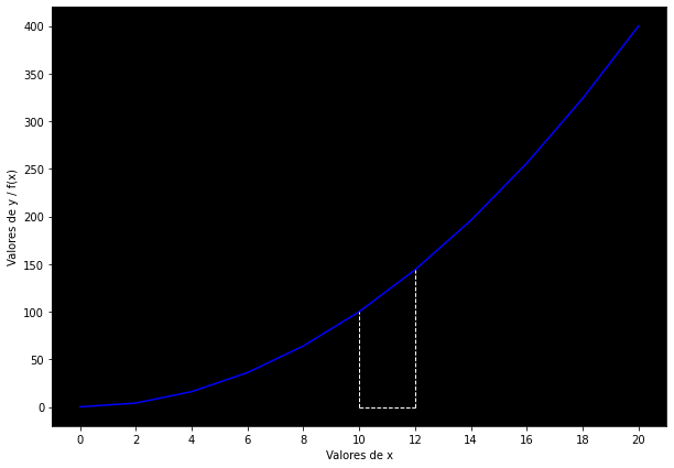
For example, let’s say I have the following quadratic function and I wish to obtain the area of the segment denoted by the dotted lines:

x = np.arange(0, 21, 2)
def f(x): return x**2
y = f(x)

A possible approximation could be obtained through the areas of the rectangle and the triangle that can be formed below:

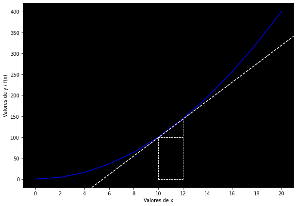
Where:

\text{Rectangle} = base \times height = x \cdot f(x) = (12 - 10)(100) = 200

\text{Triangle} = \frac{1}{2} \times base \times height = \frac{x \cdot f(x)}{2} = \frac{(12-10)(144-100)}{2} = 44

\text{Total area} = 200+44 = 244

But we could also think of a simpler approximation, although slightly less exact, namely, determining only the area of the rectangle that occupies that area:

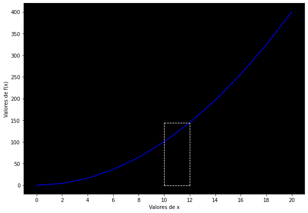
Resulting in:

\text{Rectangle} = x \cdot f(x) = (12 - 10)(144) = 288

However, we know that these calculations are inexact and laborious. We also know that functions can take more complex forms where the procedure of drawing figures would be laborious and inefficient. At the same time, the “tricks” of differential calculus can suggest to us that a solution must exist. What if we start by approximating the correct number with smaller rectangles?

x = np.arange(0, 21, 0.5)
def f(x): return x**2
y = f(x)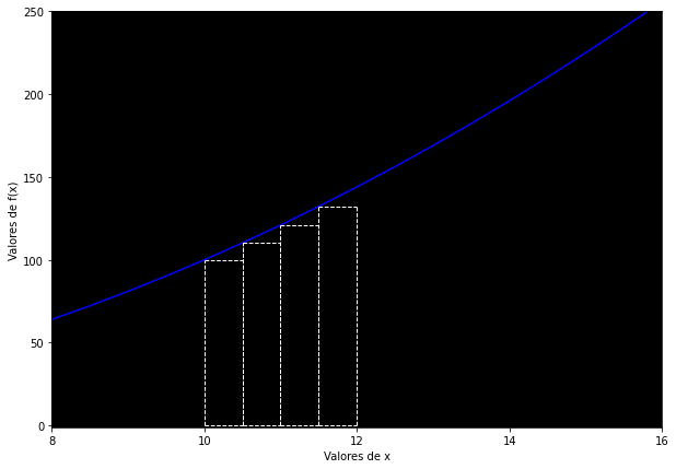

Now I have four rectangles with a base of 0.5, whose areas I can determine as follows:

\text{Rectangle 1} = x_1 \cdot f(x_1) = (10.5 - 10)(100) = 50 \\ \text{Rectangle 2} = x_2 \cdot f(x_2) = (11 - 10.5)(121) = 60.5 \\ \text{Rectangle 3} = x_3 \cdot f(x_3) = (11.5 - 10.5)(132.25) = 66.12 \\ \text{Rectangle 4} = x_4 \cdot f(x_4) = (12 - 11.5)(144) = 72 \\

Finally, to obtain the total area, I sum all the values together: 50+60.5+66.12+72 = 248.62

We have approximated the result better and our number looks similar to our first calculation. Now, to fully enter the realm of infinitesimal calculus, we need to engage with the paradoxical and tangled world of the infinite. Would a result not be more accurate if we used 10 rectangles instead of 4? Better yet, why not use a thousand, a million, or, even better, infinitely many rectangles to perform our calculation? That is the essence of integral calculus and, already familiar with the derivative, it may seem reasonable and intuitive to us.

Let’s try it programmatically, since doing it manually would be a disaster. Let’s obtain 2100 values of x, from 0 to 20.999 in intervals of 0.01:

x = np.arange(0, 21, 0.01)
def f(x): return x**2
y = f(x)

In the same way, we obtain their corresponding y values with f(x) = x^2. To obtain the area within the coordinates (x_1=10, y_1=100), (x_2=12, y_2=144), we can obtain hundreds of rectangles with a base or distance between the x’s of 0.01. The height of each rectangle will be the value of y that corresponds to the x in question.

We will multiply each of these heights by a base x of 0.01 to obtain the area of each mini rectangle. Finally, we will sum all these individual areas together to obtain the total area. This operation is called a Riemann sum, and mathematically it is expressed as:

\lim_{\Delta x \to 0} \sum_{i=1}^{n} f(x_i)\Delta x

where f(x_i) is the value of the function at the i-th point, \Delta x is the width of the rectangle, and n is the number of rectangles. Programmatically, it translates to:

sum(y[1000:1200])*0.01

~ 242.4467000000001

Graphically, our journey has been more or less like this:

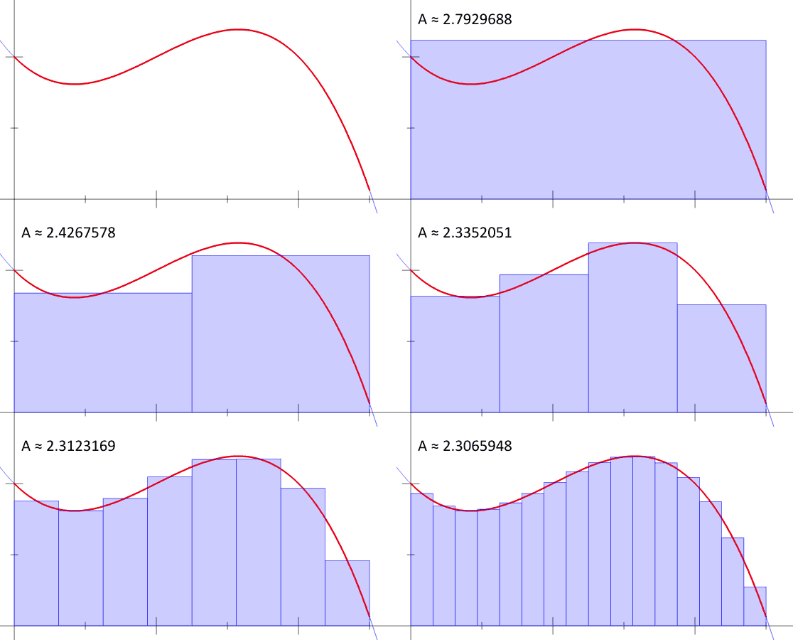
Shout out to Bernhard Riemann.

Our experiment has been successful and we have obtained the best result so far. Before continuing, let’s pause a moment to ground our ideas, formalize them, and verify that our work is correct.

So far, we have said that the area of each of the infinitely thin rectangles we have suggested is equal to the height (that is, f(x)) multiplied by the base, which in this case would be an infinitely small distance or difference between the x’s, that is, close to 0, just as with derivatives; but now, instead of using h to express this idea, we will use dx because it better expresses the idea of a small difference between the x’s.

In that sense, we have that each area of our rectangles is f(x) \cdot dx. Finally, to integrate or sum together all these small areas and obtain the total area, we can use an elongated letter “s”: \int. We will also indicate that this sum will be performed with the areas of all rectangles from x_1 to x_n or, to avoid confusion with so many x’s, from a to b, obtaining the following expression:

\int_{a}^{b}f(x) \cdot dx

In reality, to be able to use this formula we need the fundamental theorem of calculus. This theorem, which is too cumbersome to understand in detail, tells us that differentiation (derivatives) and integration (integrals) are inverse operations, much like division and multiplication. Let’s settle for that for now. And, that being the case, let’s understand that we can use the “antiderivative”¹ (the inverse of the derivative) to solve an integral. That is, if the derivative and the integral are inverse operations, then we simply invert a derivative and that should give us the result of the integral. For example, if the derivative of x^n with respect to x is {nx}^{n-1}, then the antiderivative or integral of x^n with respect to x is \frac{x^{n+1}}{n+1}+C². That is, instead of subtracting 1 from the exponent, we add 1; and instead of multiplying by the exponent, we divide by the exponent. Then we add the constant and voila.

Now, to use this formula, we simply replace the values of the interval [a, b] that interest us (in this case, from point 10 to 12), replace f(x) with the value of the function, and obtain the antiderivative (which we will denote by F) of the function at a and b, to finally subtract the antiderivatives from each other. (Let us be clear: the antiderivative measures the area under the curve of the function from the origin, 0, to x; therefore, F(b), the antiderivative of b, that is, of 12, measures the area under the curve of the function from 0 to 12. But if we are only interested in the area from point 10 to point 12, we can subtract the area of F(a), from 0 to 10, from the area of F(b), from 0 to 12, and that’s it).

\int_{a}^{b}f(x)dx = F(b) - F(a)

\int_{a}^{b}f(x)dx = \int_{10}^{12} x^2 dx

F(x^2) = \frac{x^{n+1}}{n+1}+C = \frac{x^{2+1}}{2+1}+C = \frac{x^3}{3}

\int_{a=10}^{b=12}(x^2)dx = \left(\frac{b^{n+1}}{n+1}+C\right) - \left(\frac{a^{n+1}}{n+1}+C\right) = \frac{12^3}{3} - \frac{10^3}{3} = 576-333.33 = 242.67

Reflections

Curiously, the word “calculus” comes from the Latin calculus, whose meaning is “small stone.” Calculating, in ancient times, implied the use of small stones that were counted one after another, just as when we were children we did with the abacus.

Calculus deals with infinitely small changes, hence its name “infinitesimal calculus.” Initially, these “small changes” were conceived as practical tricks that facilitated calculations like the ones we have done, but there was never a mathematically rigorous justification for proceeding this way, “imagining” infinitely small figures. That is precisely why Newton refused to publish his calculus work and why Leibniz affirmed that dealing with the infinitely small was a simple mental fiction that facilitated certain calculations in practice. That is also why ideas like an “infinitely small secant that merges with a point” sound like a paradox.

My intention in these lessons has been to plant an elementary, intuitive, and conceptual understanding of infinitesimal calculus. In my judgment, this type of rational understanding (grounded in the causes of things), besides being the most important, is conspicuously absent in the unfortunate majority of schools, books, lessons, and mathematics lectures.

Complementing these lessons with the study of certain rules for differentiation or integration is quite simple, while proceeding inversely is incredibly difficult. Intuiting the reasons behind each detail in an abstract mathematical formula (written with Greek symbols, italics, and archaic letters) is, at most, possible after years of training in the dark arts and depths of mathematics; however, when teaching mathematics, the educational system and mathematicians assume that any young student, without any motivation to do so, is perfectly capable of such a feat. I consider this a resounding failure and my work has been a humble attempt to remedy it in some way.

References

During the writing of my texts on derivatives and integrals, in addition to Khan Academy courses, the following YouTube videos were particularly useful:

• Eddie Woo’s lessons on differential and integral calculus.
• This Is the Calculus They Won’t Teach You by A Well-Rested Dog.
• Why is calculus so… EASY? by Mathologer.
• Understand Calculus in 35 Minutes by The Organic Chemistry Tutor.

As I recall, the lesson by Traductor de Ingenieria on derivatives has a good approach, though it tends to make things more complicated than they are. Similarly, 3Blue1Brown’s videos, though good at times, always confuse me and leave gaps between ideas. In any case, both deserve a mention.

Finally, although I have only skimmed a few pages, it seems to me that Calculus made easy by Thompson is a good book.