Blog — Mathematical principlesDante Noguez |
Version | 0.5.0 | |
|---|---|---|---|
| Lan | ES/IT | ||
The master Corominas has observed that, etymologically, the word “function” refers to the ‘fulfillment’ or ‘execution (of something)’. In common speech, we use this idea to refer to the task that an instrument, entity, or person is supposed to perform. Although with subtle differences, this idea of “function” also underlies mathematics, computer science, programming languages, and artificial intelligence. “Function” is a term so elementary for all these disciplines and so intuitive to all of us in everyday speech, that we will use it as a basis in this text to understand the very rudiments of these disciplines.
When we talk about the “function (of something)” in everyday life, we can say that we are referring to the operation that is performed on an object to obtain a desired result. The function of a refrigerator, for example, is to maintain a certain temperature inside, that is, to refrigerate. As a result, the food we store in it is kept in good condition. Following this line, we can schematize the function of the refrigerator (“refrigeration”) as follows:
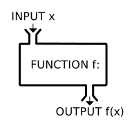
Food → Refrigeration → Food preservationIllustratively, we can also represent this scheme in the following form:
Where from the generalization of the initial scheme, it follows that the function denotes the operation or series of operations that are performed on an “input” value (in our example, the food) to result in an “output” value (the preservation of the food at a low temperature). In other words, the core of a function is to define one or more operations that are performed with the input value to transform it in some way and result in an output value. Let’s take several examples to better assimilate this:
Input → Function ("computation", "algorithm") → Output
Ingredients → Recipe (preparation) → Pizza
Book → Reading (interpretation) → Learning
Investment → Production → Business
Hypothesis → Experimentation → Scientific discovery
Law (Legislative Branch) → Interpretation (Judicial B.) → Execution (Executive B.)
In turn, any of these functions can be broken down into many others. For example, we can break down each part of the previous state paradigm according to the internal functioning of each Branch:
Proposed law → Review (voting, approval) → New law
Law → Interpretation → Judgment, jurisprudence
Judgment → Execution of the judgment → Justice
As I was saying, this paradigmatic (model, base) way of understanding the function will give us the key to understanding an infinity of concepts and phenomena in a number of disciplines. In reality, the genesis of this idea of function is in mathematics. More particularly, in a 1673 manuscript penned by the great Gottfried Leibniz, which is titled Methodus tangentium inversa seu de functionibus (“the inverse method of tangents, or on functions”).1 2
Developed further by another colossus (our master Leonhard Euler), this understanding of the function has precisely the same meaning that we have been giving it. To not lose rigor, let’s briefly specify what we mean. Although there are different ways to define a mathematical function, let’s use the most common one: the function is a unique relationship of dependence between an element of one set and another element of another set.
Let’s go step by step: sets are groups or collections of numbers, elements, or objects with common characteristics. The even numbers, for example, can be understood as a set: \{2, 4, 6, ...\}. The definition of the set “even numbers” clearly expresses that said set can only contain numbers that have two as a multiple.
Then, it is said that there is a relationship between elements of one set with elements of another. Following our example, I can say that the set \{6, 12, 18, ...\} is related to the set of even numbers by a multiplication by the number 3. Thus, the set of even numbers would be the input, and this second set would be the output. In that sense, the relationship between the elements of both sets is given according to the rules or operations that a function defines (in this case, a multiplication by 3). Each output value depends entirely on the operations performed with the input value, and this dependence is unique because each input value can only correspond to one output value. It is impossible, for example, for the number 2 as an input value to correspond to the numbers 7, 10, and 24 of the output set, since 2 \times 3 = 6, so that exclusively the number 6 of the output set corresponds to 2. In a word: multiplication is a function, and when we multiply we can only have a single valid result as an answer.
In mathematics, we will also see that the notation and representation of a function have a particular form. The most common mathematical notation to denote a function is f(x); its most common representation is a graph with Cartesian coordinates. Let’s exemplify with the case f(x) = x^{2}. According to our scheme, the input is any number (which we will represent with an x), the operation (function) that we will perform on it is to square it, which will result in (output) another number, which we can call with the letter y3:
\ x \to f(x) \to y \\ \ x \to x^{2} \to y \\
The fact that this mathematical notation may seem confusing to us is due to its level of abstraction. In reality, the use of letters (x, y, etc.) instead of numbers is an academic convention used to facilitate the definition of general rules. These letters communicate to the reader that they are variables, that is, that their value can vary depending on the context. Mathematics always demands the generalization of the formulations and expressions of its field, so that this type of “technicality” is indispensable. Otherwise, it would be incredibly laborious (and even confusing) to write complex mathematical expressions in a different style (e.g., “if we have a mathematical function of any number that is equal to said number squared”) than the traditional f(x) = x^{2} (read: “f of x equals x squared”).
Sometimes, the function is accompanied by the definition of its domain, that is, it can be indicated what type of object the input that we will introduce into the function is. For example:
\ f(x) = x^{2}, \ \ \ x\in\mathbb{R}\
Where \in means “belongs to” and \mathbb{R} is used to represent the real numbers. Then we would read the last expression as “where x belongs to the set of real numbers”.
An elementary principle of communication is the economy of language: language should always be as clear and simple as possible. Paradoxically, this notation is the simplest that exists, and any other way of communicating mathematical formulas would be inefficient and confusing. In reality, mathematical notation only seems strange to us due to lack of habit, and that is completely normal.
Returning to our topic, let’s finally see the graphical representation of a mathematical function:
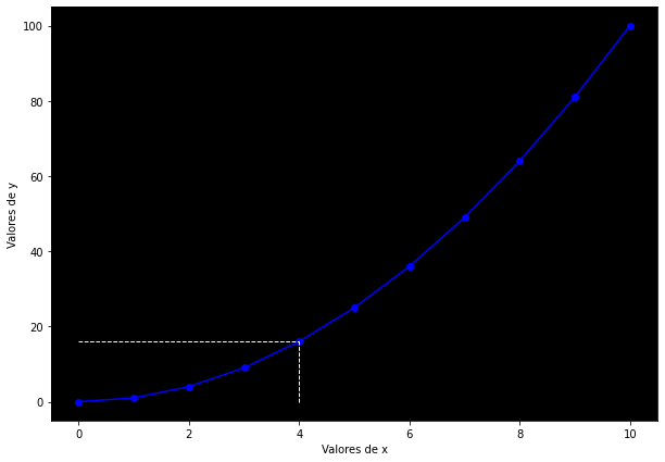
In the previous graph, the horizontal axis represents the values of x; the vertical, those of y. What each point tells us is that, for example, when x is 2, then y is 4; when x is 4, then y is 16; and so on. This is because our function indicates that y is the result of squaring x. Finally, we draw a blue line that connects all the points to represent the trend they follow; similarly, we draw a dotted white line to randomly point out an intersection of the x’s with the y’s.
We can also represent this as a table:
| Values of x | Values of y |
|---|---|
| 0 | 0 |
| 1 | 1 |
| 2 | 4 |
| 3 | 9 |
| 4 | 16 |
| 5 | 25 |
| 6 | 36 |
| 7 | 49 |
| 8 | 64 |
| 9 | 81 |
| 10 | 100 |
As you can see, our y values are the result of the function f(x) = x^2. The x takes the value of each number from 0 to 10 and, as a consequence, the operation that defines the function is performed on it to finally give a result. Let’s show some equivalences again:
\ x \to f(x) \to y \\ \ x \to x^2 \to y \\ \ 2 \to 2^2 \to 4 \\ \ 4 \to 4^2 \to 16 \\ \ 5 \to 5^2 \to 25 \\
The function is exactly the same in mathematical notation, in programmatic notation, in the graph we made, in the little table above, and in this last scheme. In the end, we are only using different signs proper to our languages (numbers, letters, lines, arrows) to represent the same thing in different ways. All these forms of representation are valid, but we will use one or another depending on the context and our own taste.
At this point, it is worth noting that “abstract” is, by definition, a way of symbolically representing ideas or objects from reality. Etymologically, the word “abstract” is composed of ab- (“to move away”, “away from something”) and trahēre (“to drag”, “to pull from something”), so that “to abstract” means to drag something out of its original form. To abstract, then, implies separating something from its other parts or from its initial situation to represent it in another way. In arithmetic, for example, the numerical properties are separated from the chromatic, sensory, chemical, nutritional properties of two pairs of apples to represent (and even generalize) in an abstract way (i.e., by means of signs “2, +, 4”) the strictly mathematical properties of those two pairs, as 2 + 2 = 4.
At some point, the numerical properties of different objects became consolidated in such a way that a new science was constituted, dissociated from our personal criteria and from the concrete physical forms of our environment. This new science, sovereign over its own field, was and continues to be today capable of discovering new mathematical configurations through the relationships and operations that can occur within itself, without explicit attention to the reality that surrounds it; but this “artificial” or formal process should never lead us to believe that mathematical operations have to do with realities different from ours. All possible thought, whether scientific, delusional, or fanciful, always originates on the surface of the earth, no matter how much our elaborate systems of thought may appear to the contrary.
To learn more about forms of representation, read Poetizar by Gustavo Bueno.
Graphing functions
Finally, I would like to use this new learning to strengthen our intuition about graphing functions. That is, we will see why the quadratic function is a parabola, why the sigmoid looks like the letter S, and so on. This has to do with the behavior of the function: the graph represents the pattern that (thanks to the function) results from the intersections between the values of x and the values of y.
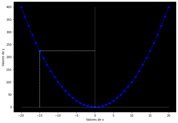
A cubic function:
\ \operatorname{Cubic}(x) = x^3
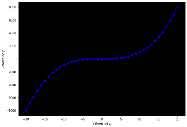
The ReLU (Rectified Linear Unit) activation function, widely used in deep learning, is defined as:
\ ReLU(x) = max(0, x)
Its function is to convert all negative numbers to 0 and reserve their original value for positive ones. In the formula we can see that for each number that enters the function, the result is the maximum value between 0 and the input value: if the input value is -1, then the result is 0 (because 0 is greater than -1); similarly, if the input value is 1, then the result will be 1 (because 1 > 0).
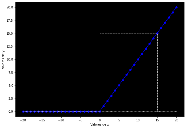
We can even graph functions that might seem like hieroglyphics mathematically, but are quite simple programmatically. The softmax function is given by:
\ Softmax(x_i) = \frac{e^{x_i}}{\sum_{j=1}^{K} e^{x_j}}\
To understand it better, we can break down its terms:
| Notation | Interpretation |
|---|---|
| x_i | Each corresponding value of x, “the i-th value of x” |
| e | Euler’s number, is equal to 2.71828 |
| e^{x_i} | Euler’s number raised to the corresponding value of x |
| \sum | Summation: indicates that all the accompanying values must be added together; this symbol is a letter S (“sigma”) in the Greek alphabet |
| _{j=1} | Indicates the value from which the summation will start |
| K | Total number of values of x |
| \sum_{j=1}^{K} e^{x_j} | The summation must be performed on all the values of e^{x_j} that we have, that is, starting with the first value of x (i.e., x_j) and ending at the value x_K (i.e., the last value of x). |
In simple terms, this formula says that the softmax function consists of dividing the number e raised to the power of x_i (that is, to the power of the corresponding value of x) by the summation of all the values of x as powers of the number e. If we were to write it out step by step, it would look like this:
\ Softmax(x_i) = \frac{2.71828^{x_i}}{2.71828^{x_j} + 2.71828^{x_2} + 2.71828^{x_3}, ... 2.71828^{x_K}}\
Suppose our x’s are the numbers from -2 to 1, then we substitute values and apply the formula:
\ Softmax(x_1) = Softmax(-2) = \frac{2.71828^{-2}}{2.71828^{-2} + 2.71828^{-1} + 2.71828^{0} + 2.71828^{1}}\
\ Softmax(x_2) = Softmax(-1) = \frac{2.71828^{-1}}{2.71828^{-2} + 2.71828^{-1} + 2.71828^{0} + 2.71828^{1}}\
\ Softmax(x_3) = Softmax(0) = \frac{2.71828^{0}}{2.71828^{-2} + 2.71828^{-1} + 2.71828^{0} + 2.71828^{1}}\
\ Softmax(x_4) = Softmax(1) = \frac{2.71828^{1}}{2.71828^{-2} + 2.71828^{-1} + 2.71828^{0} + 2.71828^{1}}\
Our results (or y values, if you will) would be 0.032, 0.087, 0.236, and 0.643, respectively. The summed values always give 1 when we apply the softmax function to them.
Now we can better appreciate the simplicity of the initial formula, compared to the laborious breakdown we must do when calculating value by value. This is one of the reasons why mathematical notation is so abstract.
Fortunately, Python saves us all this trouble. We can delegate the calculation of this convoluted and exhausting formula to our little program:
def Softmax(x):
  return np.exp(x) / sum(np.exp(x))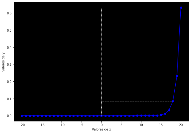
First, let’s focus on understanding that these functions imply a pattern, which defines the way we will obtain y.
Now, where does all this come from and what does it mean? The answer also depends on what we want to do with our learning. First, let’s emphasize again that all these signs are ways of representing. To discover something or talk about something new also implies the need to find a way to communicate that novelty. Naturally, communicating that novelty entails formulating new concepts, ideas, and expressions to be able to communicate it; otherwise, it would be impossible to differentiate it from what we already know.
In that sense, the first mathematicians who tried to understand the concept of function also sought a way to express it. Perhaps by chance, for ease, by the authority of the great Leonhard Euler, or for hundreds of other possible reasons, the notation that everyone finally agreed to use was f(x). Similarly, the geometric, textual, or programmatic ways of representing it are also a convention, just as these letters, accents, and commas that I write are also. The objective “decision” about which conventions remain and which others disappear is always beyond us. In any case, each person understands and represents all these things differently for themselves.
On the other hand, as I say, its use will depend on us. In the case of a function, for example, a mathematician is interested in the logical, numerical, geometric, and abstract properties of the function; a computer scientist, in knowing what a function is and how it relates to the operation of a computer; a programmer, in knowing what properties the functions of a certain language have. We can give them that or any other utility that we see fit.
Let’s say, for example, that we have just discovered that languages change at a rate that can be represented by a sigmoid function: first, no one uses the expression we want to study; at some point, a new expression appears and begins to be used by a few people; then, there comes a point where it spreads rapidly among the population; and finally, upon being universally adopted, its use changes very little, since no one stops using it, nor does anyone begin to use it for the first time.
The formula to generate a graph of this nature is:
\ Sigmoid(x) = \sigma(x) = \frac{1}{1 + e^{-x}}\
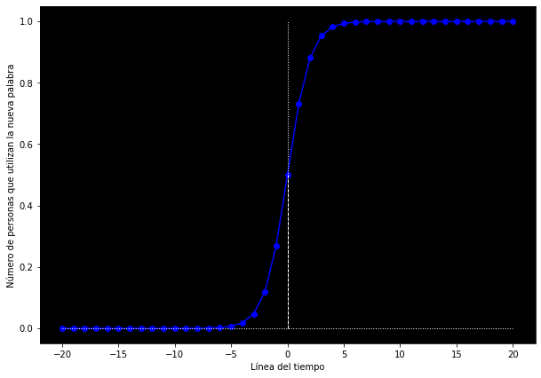
As we were saying: first nobody uses it, then a few people, then it grows rapidly and finally it stagnates. In this case, x represents the passage of time and y the number of people who use a word.
This function can be used to represent the number of people infected with COVID-19, the development of an embryo, the growth of a new industry, and thousands of other things. In the same way, it can be given more complex uses: for example, it can be used to diagnose diseases with mathematical models (artificial intelligence models). Its usefulness depends entirely on us.
To talk about algorithms, we will stick to what Donald Knuth (a prominent programmer) has sentenced about them. In essence, an algorithm consists of a finite set of ordered rules or instructions whose purpose is to solve a specific type of problem.
According to Knuth, every algorithm must offer a concrete solution to the problem it proposes to solve; in addition, it must be defined, that is, precise, not ambiguous; it must also be effective4, in the sense that the operations it contains are basic enough so that they can be performed in a finite period of time by anyone; finally, it must contain an “input” and an “output,” terms with which we are already familiar.
To illustrate this concept, we can begin with a simple example of an algorithm. Let’s say we are interested in creating an algorithm for putting on a shoe. We could sketch the following scheme:
1. Take the shoe with both hands.
2. Point the heel of the shoe towards us.
3. Put the tip of our foot inside the shoe.
4. Change the grip to hold the shoe with the thumbs inside it.
5. Put our foot to the bottom of the shoe while taking out the thumbs.
As we can see, the nature of the algorithm is quite simple, although its formulation is not easy at all. Strictly speaking, an algorithm only works when we truly satisfy the requirements we mentioned before. The algorithm for putting on shoes that we have just suggested could fail in a thousand ways: how do I distinguish the left shoe from the right? How do I choose which pair of shoes to wear? What happens if I drop the shoe from my hands during step 2? Although we can humanly improvise or reason each step, a computer cannot, so our algorithm would be useless in the face of any unforeseen event.
We could also say that, despite certain subtle differences, an algorithm and a function are the same thing: an operation performed on an input to result in an output.
That said, it seems to me that this sketch is sufficient for the moment to understand the algorithm. Although the algorithm is a kind of simple recipe or instruction to solve a concrete problem, its complexity lies in the meticulous level of detail it requires to be effective. In my opinion, the algorithm is the mechanical use of brute force to achieve an end; but that brute force must be meticulously calibrated.
Finally, let’s exemplify with a true algorithm. We will formulate the famous Euclid’s algorithm, used to find the greatest common divisor of two numbers.
Although the algorithmic notation may be more familiar to us, it is necessary to warn that the “←” sign can be confusing because it indicates a sequence from right to left. This sign indicates that the value on the left acquires the value on the right: “n ← r” means “n acquires the value of r”; the “↔︎” sign, on the other hand, means that we must exchange the value of the variables with each other.
Now, the algorithm: Given two positive integers m and n, Algorithm E (from Euclid) will find the greatest common divisor between them, that is, it will find the largest positive integer that can divide both without any remainder.
Algorithm E:
E0. Check that m \geq n. If m < n, exchange m \leftrightarrow n.
E1. Find the remainder. Divide m by n; the remainder will be r. (We will have that 0 \leq r < n).
E2. Is it zero? If r = 0, the algorithm ends; n is the answer.
E3. Reduce. Now m \leftarrow n, n \leftarrow r, and we will go back to step E1.
In pseudocode:
Function AlgorithmE(m, n):

If m is less than n:
  exchange values
  r = m modulo n
  if r is equal to 0:
    the result is n
  otherwise:
    while r is not equal to zero:
      exchange the values of m, n for those of n, r
      r = m modulo n
      if r is equal to 0:
        the result is n
The algorithm imposes conditions, rules, and anticipates certain situations to function. Although the “mathematical environment” is much more predictable than the “vital” one (that is, in the last algorithm we could drop the shoe, but in this algorithm no number will disappear), the truth is that even formulating algorithms of this nature is a minor art that requires some practice.
In Python, we could program it as follows:
def AlgorithmE(m, n):
  if m < n:
    m, n = n, m
  r = m%n
  if r == 0:
    return n
  else:
    while r != 0:
      m, n = n, r
      r = m%n
      if r == 0:
        return n
# A simplified version of the algorithm:
def Euclid(a, b):
while b != 0:
a, b = b, a % b
return a# We test the algorithms:
results_1 = AlgorithmE(544, 119), AlgorithmE(2166, 6099)
results_2 = Euclid(544, 119), Euclid(2166, 6099)
print(f'Results of the first algorithm: {results_1} | Results of the second algorithm: {results_2}')In my opinion, the most important algorithm in history is the Turing machine. This algorithm defined a model for the computers of our day, and its simplicity is as impressive as its capability.
To know what that algorithm consists of, read: The Annotated Turing by Petzold.
Among other things, for us the interest of the algorithm or the function lies precisely in that they allow us to understand the potential of the most advanced machine of our days. Programming, for its part, allows us to materialize or take advantage of that understanding.
In essence, programming implies communicating instructions (algorithms, functions) to a computer. The instructions formulated in a programming language are translated by means of a compiler (that is, another program) into “machine language,” that is, into a binary system that can then be “interpreted” by the transistors of the microprocessor.
As is known, the binary system used by computers consists of zeros and ones. For example, the numbers from 0 to 8 would be5:
0. 0 0 0
1. 0 0 1
2. 0 1 0
3. 0 1 1
4. 1 0 0
5. 1 0 1
6. 1 1 0
7. 1 1 1
8. 1 0 0 0
Let’s take the following number from the decimal system:
1 \ 2 \ 3
Here, the 3 is in the units place; the two, in the tens; and the one, in the hundreds. So,
(100 \times 1) + (10 \times 2) + (1 \times 3) = 100 + 20 + 3 = 123
Each place of each digit represents a power of 10, so there are ten possible digits in each place (now the term “decimal system” begins to make sense). The first place from the right represents a 10^0; the one in the middle, 10^1; the third, 10^2, and so on:
\ 10^2\ 10^1\ 10^0\ \\ 1 \ \ \ \ \ \ \ 2 \ \ \ \ \ \ \ 3
In binary, on the other hand, we only have two digits and the exponents of two in each place:
\ ... 2^2\ 2^1\ 2^0\
Which is equivalent to:
\ ... 4\ 2\ 1\
So, if we wanted to represent the decimal value 3, we would have to add 2 and 1 in the binary system like this:
\ 2^2\ 2^1\ 2^0\ \\ 0 \ \ \ \ 1 \ \ \ \ 1
And the decimal value 123:
\ 2^6 \ 2^5\ 2^4\ 2^3 \ 2^2\ 2^1\ 2^0 \ \\ 1 \ \ 1 \ \ 1 \ \ 1 \ \ 0 \ \ 1 \ \ 1
Most computers use 8 digits or bits (which means “binary digit”) at a time, so the number 3 would be 00000011. Each set of 8 bits is called a byte.
Although the decimal system prevails in humans for being more intuitive to us, the truth is that once again we are talking about a convention. Xul Solar, for example, was a singular man who for a long time maintained that the duodecimal system of numeration is superior to the decimal. In his personal and professional life, Xul Solar used that system.
The binary system, on the other hand, is especially convenient for computers for the simple reason that it facilitates the translation of zeros and ones into electrical signals: zero indicates off; one, on. The transistor fulfills the function of electrically representing the ones and zeros of the computer, performing operations with them by continuously turning on and off. A computer processor is composed of millions of transistors representing ones and zeros. A transistor can represent hundreds of billions of zeros and ones per second; the smallest transistor of our day is about 50,000 times thinner than a hair.
The binary system was formulated by none other than our old friend Leibniz, who also probably used the term “algorithm” in a modern sense for the first time. Leibniz was a colleague of Johann Bernoulli, who in turn was a mentor to our other friend Leonhard Euler.
Naturally, the binary system, in addition to representing numbers, can also represent letters, images, videos, music, and everything we see on a computer screen. For this, different combinations of binary code have been agreed upon to represent certain characters. The letter “A,” for example, is represented by the number 65, which in binary is 01000001; ASCII and Unicode are standard codes for representing the alphabet and some special characters.
On the other hand, the standard for representing colors is RGB, which indicates the amount of red, green, and blue that the color to be represented contains. Each pixel on computer screens uses three bytes to represent a color.
As we get closer to an image, we can better see the pixels (the small colored squares) that represent it. Thus, we already know that the most powerful machine created by humans consists of enormous sequences of numbers.
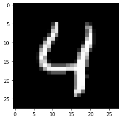
The problem lies precisely in that: these sequences are gigantic, so communicating with the computer in that language would be a torment. Therefore, programming languages facilitate said communication, since the computer knows how to translate into its language the instructions we give it through a program. As we will see later, only a few lines of code are necessary to create an artificial intelligence program.
Cf. Herrera Castillo (2013) and Scriba (1964).↩︎
Leibniz not only coined the term “function”, but also “variable”, “constant”, “coordinate”, “differential equation”. In the words of Dietrich Mahnke (whom, by the way, we also mention in our text regarding Borges), this valuable manuscript by Leibniz already contained the germ of several important concepts of modern mathematics: the Taylor series, infinitesimal calculus, and functions.↩︎
Functions can also be written using a mapping arrow, such as: x \mapsto x^2, which is equivalent to our example f(x) = x^{2}. However, it is preferable to get used to this last way of formulating them, since it is the most common.↩︎
The “effectiveness” to which Knuth refers is similar to the “independence” to which David Hilbert referred when he spoke of “axiomatic thought”: the axioms of a system must be such that there is none that is unnecessary or superfluous, none that can be derived from another. The same could be said of algorithms.↩︎
The additional zeros to 0, 1, 2, and 3 are not necessary, but we use them to facilitate reading.↩︎